grandem_document

1 Introduction

The Gran-DEM particle flow simulator is a commercial particle flow DISCRETE ELEMENT METHOD (DEM) application that can be used to simulate particle flow in any type of pre-designed 3-D domain. This 3-D domain can be a mesh file (.msh) imported into the Gran-DEM application. The Gran-DEM application set-up (version 1.0) can be licensed and downloaded from (gran-dem.com) and installed. The procedure to do this is provided hereby;The application can next be started from the start menu. The Gran-DEM particle flow simulator is operated using a tailor developed User interface for easy formulation and set-up. The Gran-DEM UI opens immediately after starting it from the start menu. The UI design consists of 3 vertical panes LEFT (red), MIDDLE (green) and RIGHT (blue) and a horizontal TOP (orange) pane that can be seen in Fig 1.1. The UI set-up consists of 7 main functionalities organized sequentially in the left most pane of the UI. These main functionalities are SELECT MODEL, MATERIALS, SYSTEM, PARTICLE MODEL, PARTICLE INJECTION, FLUID FLOWSOLVER, BOUNDARY CONDITIONS, MONITORS, USER DEFINED FUNCTIONS, EXECUTE AND PARAVIEW VISUALIZATION.Fig. 1.1: UI layout design and its main subdivided functionalities.When any of the above main functionalities is selected the sub-selections for these appear in the middle pane. The right large pane is used for visualization. The top pane (orange) consists of File, Edit, Source, Filters, Tools and Help that are described later in Section 8.1. In the following sections various aspects of the UI operations are discussed sequentially.

2 Select Model

2.1 Description and theory:

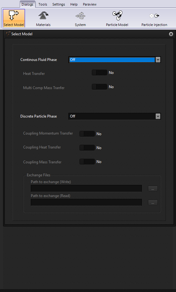
The LnE multiphase CFD simulator is a multipurpose tool for carrying out both Lagrangian (granular) and Eulerian (Fluid) flow simulations in various flexible combinations. The Eulerian (fluid) flow modelling is done by using the coupled pressure-velocity model that involves fundamentally the continuity Equation and Navier Stokes Equation solved on a 3D grid domain.Within the CFD framework this is also called the SIMPLE algorithm that stands for Semi-Implicit Method for Pressure Linked Equation proposed by Spalding and Patankar (1978). Typically, most commercial CFD solvers for unstructured grid domains use the finite volume method where the pressure and velocities are collocated at cell centre positions. However, the formulation used here is a staggered grid approach where the scalars, like pressure is defined at cell centre and vectors like velocity is defined at face centre (or staggered) position. The Single phase Eulerian can be solved with or without heat transfer (energy balance) and multi-component mass transfer.The Lagrangian particle flow modelling uses the Discrete Element Method (DEM) for treating collision mechanism. The Eulerian fluid flowsolver can be coupled 2-ways for momentum transfer or exchange with discrete particle phase or DEM. Additionally if heat and mass transfer with the fluid phase is to be initiated then it can be done.

Fig. 2.1: Select Model left pane showing fluid and particle phase model selectionAnother feature of Gran-dem is its DEM can be coupled with external software such as ANSYS FLUENT fluid flowsolver. This coupling can be done for all 3 aspects i.e. momentum, heat and mass transfer.

2.2 Setting up:

On the Main UI ‘Select Model’ setting from the left pane. Under the continuous phase drop down menu election for the Eulerian fluid flow method can be made or set off.If Fixed field, single phase Eulerian or single phase External (Fluent) is selected the user can switch on the fluid heat transfer and/or mass transfer model.If the DEM method in discrete particle phase is switched on the user can choose to couple ‘Momentum transfer’, ‘Heat transfer’ and/or ‘Mass transfer’ with the fluid phase (Eulerian) using the switches below it (Refer Fig. 2.1).If the user wants to use this feature ‘momentum transfer’ is mandatory but the remaining 2 can be chosen.If single phase External (Fluent) has been selected in the continuous phase the user should add the path to the exchange directory at the bottom of the left pane Fig. 2.1. This is needed to connect with ANSYS FLUENT and exchange coupling data.

3 Materials

3.1 Description and theory:

The flow behaviour of materials is fundamentally characterised by their physical properties. Therefore, material properties of Eulerian fluids (liquid or gas) and Lagrangian particles (liquid or solid) during CFD flow simulations are extremely important while simulating system flow behavior. The Eulerian Fluid phase can be single component or multiple component. Depending on the choices made in select model for species transport components can be added to Eulerian fluids and their physical properties entered the check boxes.Similarly, the particles properties are added into in a separate section on left pane depending on if DEM has been selected in ‘Select Model’. The particle flow dramatically affect phenomena such as segregation, wettability, heat and mass transfer, etc within process systems. The fundamental properties of particle material needed for DEM simulations are density, viscosity, thermal conductivity, species diffusivity and heat capacity. Properties like viscosity are relevant only when discrete particles are actually droplets or particles are wet. Similarly, properties like thermal conductivity are relevant when heat transfer is considered or simulations are non-isothermal.

3.2 Setting up:

On the Main UI, select ‘Material Properties’ from the left pane. This causes the component materials adding additional tabs in the middle pane to appear. This consists of the buttons ‘Add component’ and ‘Delete component’.Using the ‘Add component’ button new components can be added successively which appear one below the other as ‘Component 1’, ‘Component 2’, etc. (Fig. 2.1).Under each component, check boxes are provided for adding the ‘Component name’ and ‘Molecular Weight’ of the component. It also has a switch called ‘volatile’ indicating if the component is volatile or not and a button called ‘physical properties.The ‘volatile’ switch is switch on for components that can vaporise from the Lagrangian or discrete particles into the surroundings. It is typically switched on for components like water that can vaporize and leave the discrete phase. But for components like fertilizers, aluminum, iron oxide, etc. that do not typically vaporize during DEM simulations it need not be switched on.When the ‘physical properties’ button is clicked (see Fig. 2.2) it opens a tab to enter in the properties ‘density, viscosity, thermal conductivity, species diffusivity and heat capacity’. Note that as discrete particles are in either solid or liquid phase these properties that are to be entered are in one of these phases.If the volatile switch is on, all the above mentioned (point 5) properties are duplicated to add properties in gaseous state as well. This is essential to evaluate process parameters such as vaporization rate, vapor pressure, etc.It also provides for a thermodynamic stability factor (Rm) that gives the stability coefficient between the volatile component and non-volatile component.Fig. 2.1: The component setting in the middle pane.Fig. 2.2: Insertion of physical properties of individual component without (left) and with volatility (right)

4 System

4.1 Description and theory:

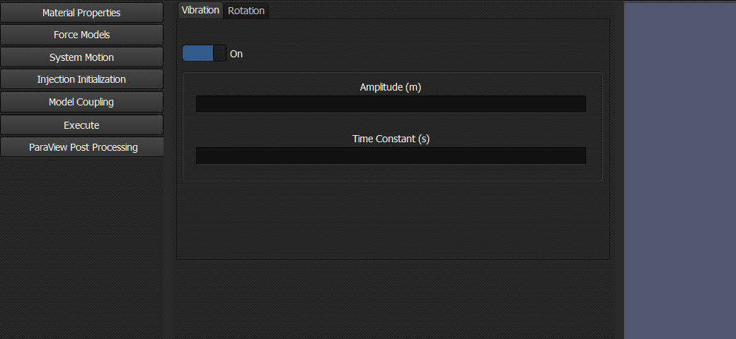
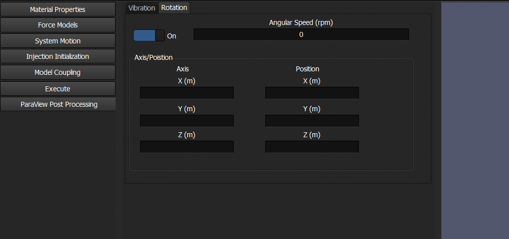
The main functionality of system motion is of relevance when DEM simulations need to be performed where the domain motion is also simulated alongside DEM particles. The domain motion here can be of two types namely; vibrational motion and rotational motion. Under this functionality the system domain or Eulerian grid consisting of nodes, cells and faces position changes dynamically with time. This begins from an original position and periodically depending on the type of motion returns to the original position.In case of vibrational motion, the entire domain including the Eulerian grid nodes, cells and faces move in a vibrational form with an amplitude and a time constant. The vibrational motion also needs to be set with vibrational direction.In case of rotational motion, the domain including the Eulerian grid nodes, cells and faces move about a position axis at a given fixed rotational speed.

4.2 Setting up:

On the Main UI, select ‘System Motion’ from the left pane. This causes 2 tabs to appear on the middle pane. The first tab to appear is the ‘Vibration’ tab as shown in Fig. 4.1.The second tab is the rotation tab which on selection the input parameters appear as shown in Fig. 4.2. Here angular speed of the system needs to be set alongside the rotation axis representing direction of axis and position representing the position through which the axis will pass. The angular rotation direction is governed by the right hand rule. So, if the axis direction is in positive z-direction the rotation will be clockwise when seen in the z-axis direction.

Fig 4.1: System motion model selection showing the vibration tab.

Fig 4.2: System motion model selection showing the rotation tab.

5 Particle Models

5.1 Description and theory:

The Discrete element method-based particle tracking is governed by Newton’s law of motion. The dynamic motion of any particle ‘a’, defined vectorially in a 3-D space by position vector ‘r_a’ and mass ‘m_a’, is determined by the sum of the forces acting on the particle. This balance is provided hereby in Eq. 3.1;

m_{a} \frac{d \vec{r_{a}}}{d t} = F_{G} + F_{C} + F_{D}

(3.1) Where;

F_{G}

is the gravity force,

F_{C}

is the contact collision force and

F_{D}

is the drag force acting on the particle.

m_{a} \frac{d \vec{r_{a}}}{d t} = F_{G} + F_{D} + F_{C}

5.1.1 Gravity force

Gravity defines the natural influence of gravitation acting on the particle mass. It is given by Eq. (3.2):

F_{G} = m_{a} \vec{g}

(3.2) Where;

\vec{g}

is the gravitational force vector defined at the center of mass of particle.

5.1.2 Collision force

Collision force is the summation of all direct contact collision forces experienced by the particle. The collision forces are treated by the soft sphere approach where a spring-dashpot method is applied. Therefore, any given particle ‘a’ can be simultaneously in collision with multiple particles ‘b’. Thus. the total collision force acting on any particle ‘a’ is sum of collision force with all contact particles ‘b’ in its contact space given by;

F_{C, a} = \sum_{b \in c o n t} F_{a b}

(3.3) Where,

F_{a b}

is the contact force due to collision between any particle ‘a’ and ‘b’. This individual force defined by the spring-dashpot method is given by;

F_{a b} = k_{n} δ_{n} \vec{n_{a b}} - η_{n} \vec{v_{a b}}

(3.4) Where;

k_{n}

is the normal spring stiffness and

η_{n}

is the normal restitution coefficient.

\vec{n_{a b}}

and

\vec{v_{a b}}

are the positional unit normal vector and relative velocity between given particles ‘a’ and ‘b’, respectively.

δ_{n}

is the prevailing contact overlap between the two particles. The normal overlap is given by;

δ_{n} = (r_{a} + r_{b}) - |\vec{r_{a}} - \vec{r_{b}}|

(3.5) Where,

\vec{r_{a}}

and

\vec{r_{b}}

represent the position vector for the colliding particles and

r_{a}

and

r_{b}

are the radii of respective particles.

5.1.3 Interphase drag force

The drag force is the force acting on particles due to fluid phase (gas or liquid) flowing around it. It is essentially the momentum transferred by the fluid phase due to friction when flowing passed the surface of the particle. This force typically can be modelled through a one way or a two-way coupling between the Lagrangian DEM phase and Eulerian fluid phase on a fixed grid. In the one way coupling only the particle phase drag is considered but in a two way coupling the drag force encountered by the fluid phase is also considered. The drag force acting on individual particle is given by;

F_{D} = β_{a} (\vec{v_{p}} - \vec{u_{p}})

(3 .6)Where;

β_{a}

is the drag coefficient,

\vec{v_{p}}

is the particle velocity vector and

\vec{u_{p}}

is the fluid velocity defined by the Eulerian grid mapped at the particle location.

5.2 Setting up:

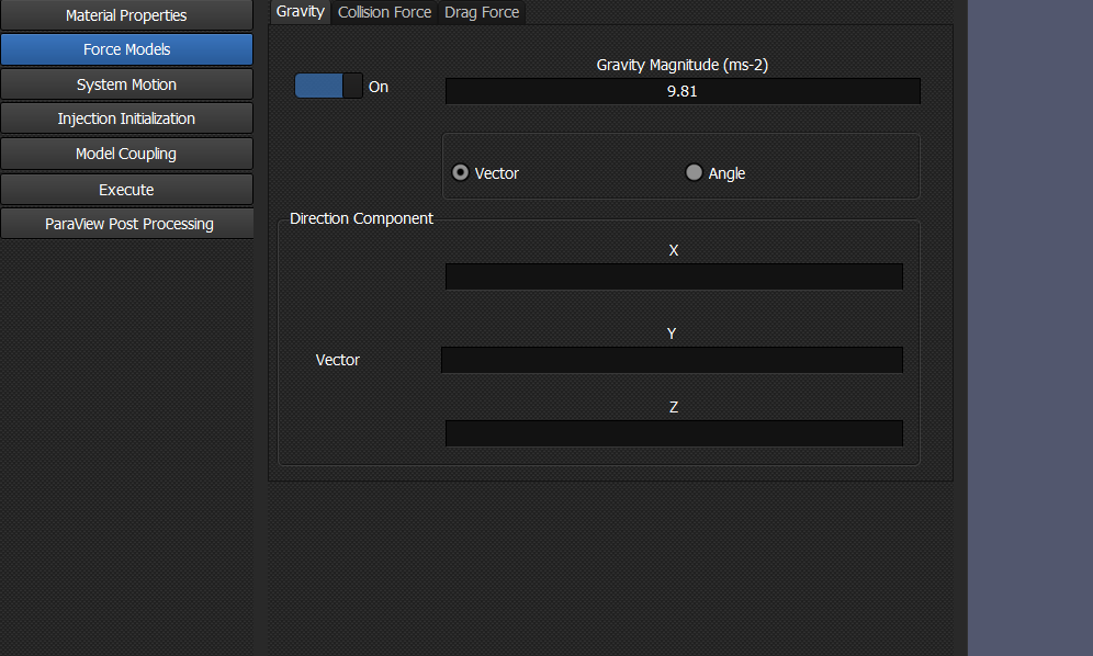
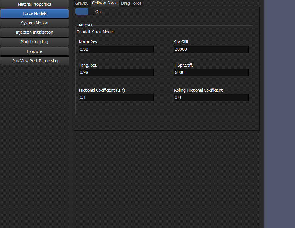
On the Main UI, select ‘Force models’ from the left pane. This causes the 3 force tabs to appear in the middle pane. The first tab to appear is the ‘gravity force’ tab as shown in Fig. 3.1.The gravity tab is default set on however user is free to deselect if needed. This tab consists of gravity magnitude dialog box where a default value of 9.81 is set and user is free to adjust as may be needed.The user has to select how the gravity direction is to be defined in the domain i.e. either vector or angular inclination. If the ‘vector’ selection is made the x, y and z component of the unit vector needs to be defined.If the ‘angle’ selection is made the angle of gravity direction with respect to xy plane and yz plane needs to be defined.The next tab is Collision force tab which is also default set “ON”. The values for various collision parameters can be set here like Normal restitution coefficient, Tangential restitution coefficient, spring stiffness, etc. as shown in Fig. 3.2.The next tab is the drag force tab, which is default OFF and needs to be switched on to use. On selection a drop-down selection panel appears using which the drag force can be chosen.

Fig 3.1: The force model selection from left tab showing the force tabs in the middle pane with gravity tab selected.

Fig 3.2: The force model selection showing the Collision force tab and its dialog boxes.

6 Injection Initialization

6.1 Description and theory:

The injection of particles into the domain is set up in this functionality. Here a flexible injection system has been provided where user is able to choose from a variety of types of injection depending on requirement. There are 4 main types of injections that can be defined. They are;Injection type 1: Specific point injectionInjection type 2: Cell centre fixed point injectionInjection type 3: Fixed square grid ordered injectionInjection type 4: Feed channel injectionPARTICLE INJECTION (FL_INJ):

6.1.1 Injection type 1: Specific point injection:

This is a completely flexible injection option provided where individual independent injection points can be defined as needed by the user. Each injection point is specified with basic variables like particle diameter, number of particles per parcel, parcel diameter, X, Y, Z position point in 3D space, X, Y, Z injection velocity in 3D space, Temperature and material composition. Besides each injection is also set with single or multiple injection. Single injection entails only 1 injection is made at time t=0.0s.If multiple injection option is chosen the user needs to additionally specify mass flow rate and its dependent variable time constant. This leads to a continuous injection of particle at a fixed time interval space. This injection is also defined in terms of mass flow rate for the given particle injection. The start and end time for injection is also defined.

6.1.2 Injection type 2: Cell centre fixed point injection:

Injection points are created at the cell centre positions of all the Eulerian grid in the system. This setting requires basic variables specified as particle diameter, number of particles per parcel, parcel diameter, X, Y, Z position point in 3D space, mean injection velocity in 3D space, Temperature and material composition. The direction of injection here is always set in the gravity direction. These variables are set for all particles injected at all cell center positions. Besides, the injection is also set with single or multiple injection. Single injection entails only 1 injection is made at time t=0.0s.If multiple injection option is chosen the user needs to additionally specify mass flow rate and its dependent variable time constant. This leads to a continuous injection of particle at a fixed time interval space. This injection is also defined in terms of mass flow rate for the given particle injection. The start and end time for injection is also defined. This injection type is typically used for filling up domain system with particles.

6.1.3 Injection type 3: Fixed square grid ordered injection:

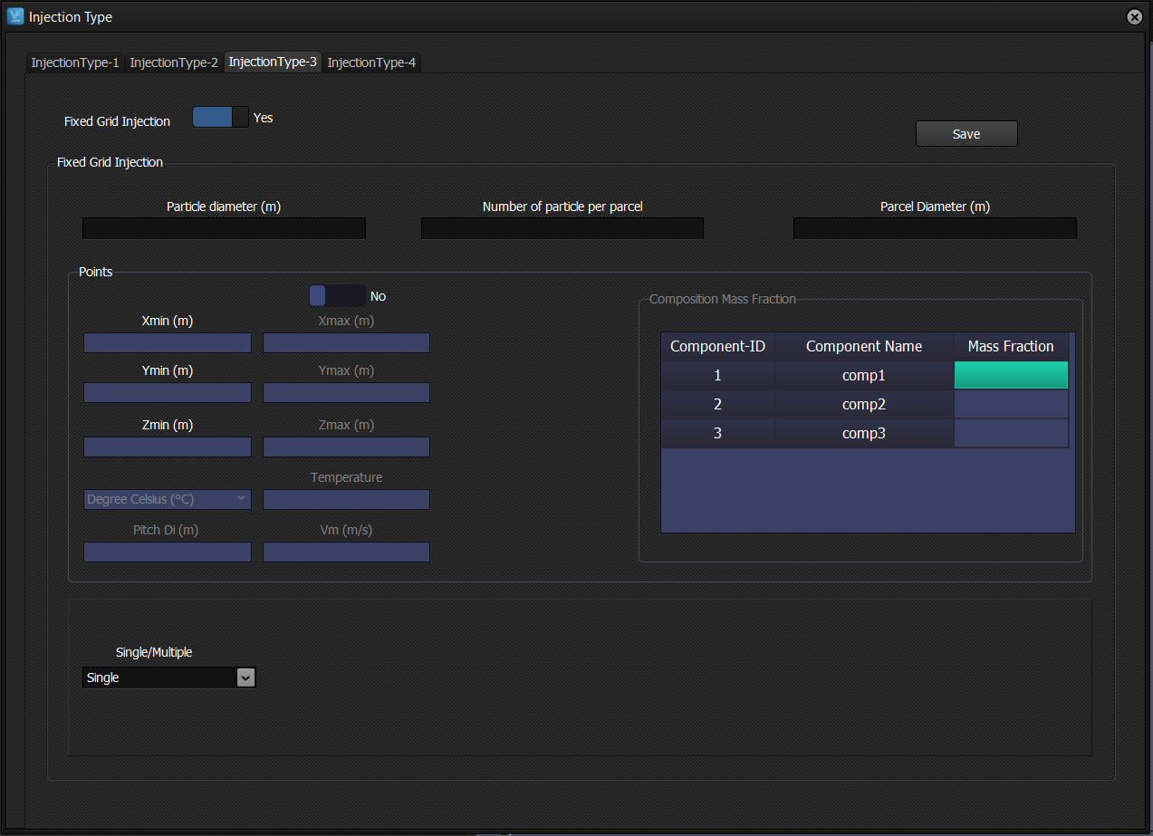
Injection points are created in a fixed square grid. This setting involves minimum and maximum positions in X,Y,Z direction and particle pitch that needs to be provided. Here the minimum and maximum can be seen as a cutoff limit in the Eulerian grid as shown in Fig. 5.1. Using this info a square grid of injection points is generated where distance between particles in each direction is the pitch. The other variables provided as usual from previous are particle diameter, number of particles per parcel, parcel diameter, X, Y, Z injection velocity in 3D space, Temperature and material composition. These variables are set for all particles injected at the square grid positions. Besides, the injection is also set with single or multiple injection. Single injection entails only 1 injection is made at time t=0.0s.Fig 5.1: Schematic showing minimum and maximum limit in an euilerian grid for limiting injection points.If multiple injection option is chosen the user needs to additionally specify mass flow rate and its dependent variable time constant. This leads to a continuous injection of particle at a fixed time interval space. This injection is also defined in terms of mass flow rate for the given particle injection. The start and end time for injection is also defined. This injection type is typically used for filling up domain system with desired amount of particles.

6.1.4 Injection type 4: Feed channel injection:

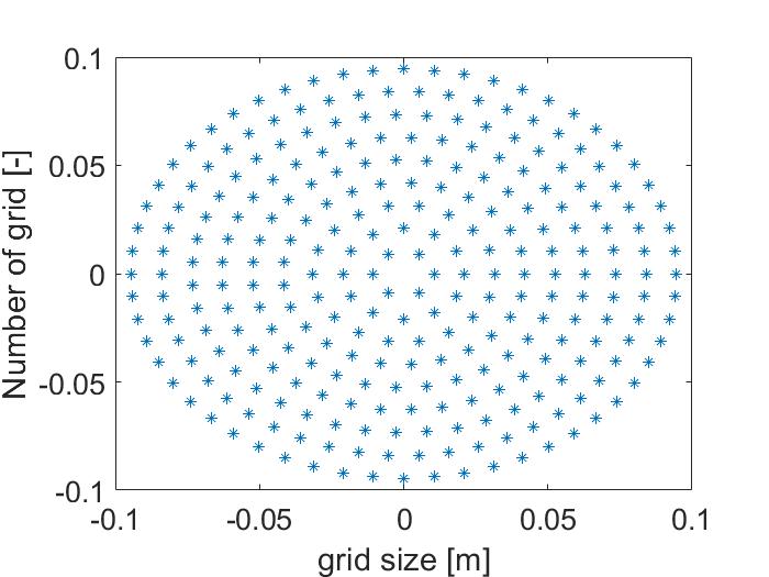
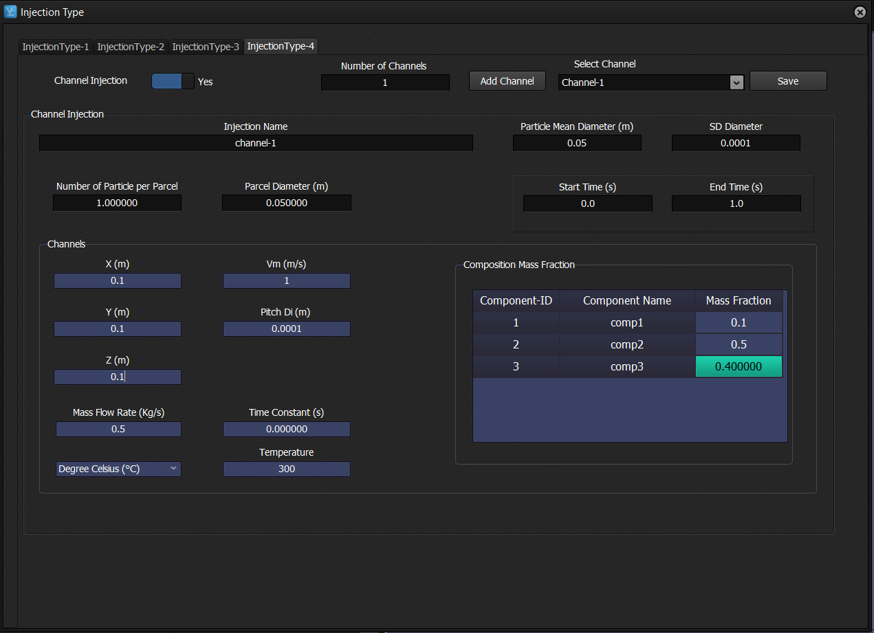
This is a special injection type where a channel feed type of injection can be defined. The injection type requires to be set with a mass flow rate, particle injection velocity and position. Using this information concentric rings of injection points are created for particulate injection. Fig. 5.2 shows a schematic of an example arranged injection points. The size of the ring depends on the mass flow rate and the pitch provided by the user. The other variables provided as usual from previous are particle diameter, number of particles per parcel, parcel diameter, X, Y, Z injection velocity in 3D space, Temperature and material composition. These variables are set for all particles injected at the square grid positions.Besides, the injection is also set with single or multiple injection. Single injection entails only 1 injection is made at time t=0.0s. If multiple injection option is chosen the user needs to additionally specify mass flow rate and its dependent variable time constant. This leads to a continuous injection of particle at a fixed time interval space. This injection is also defined in terms of mass flow rate for the given particle injection. The start and end time for injection is also defined. This injection type is typically used for filling up domain system with particles.

Fig 5.2: Feed stream channel injection arrangement in a ring form.

6.2 Setting up:

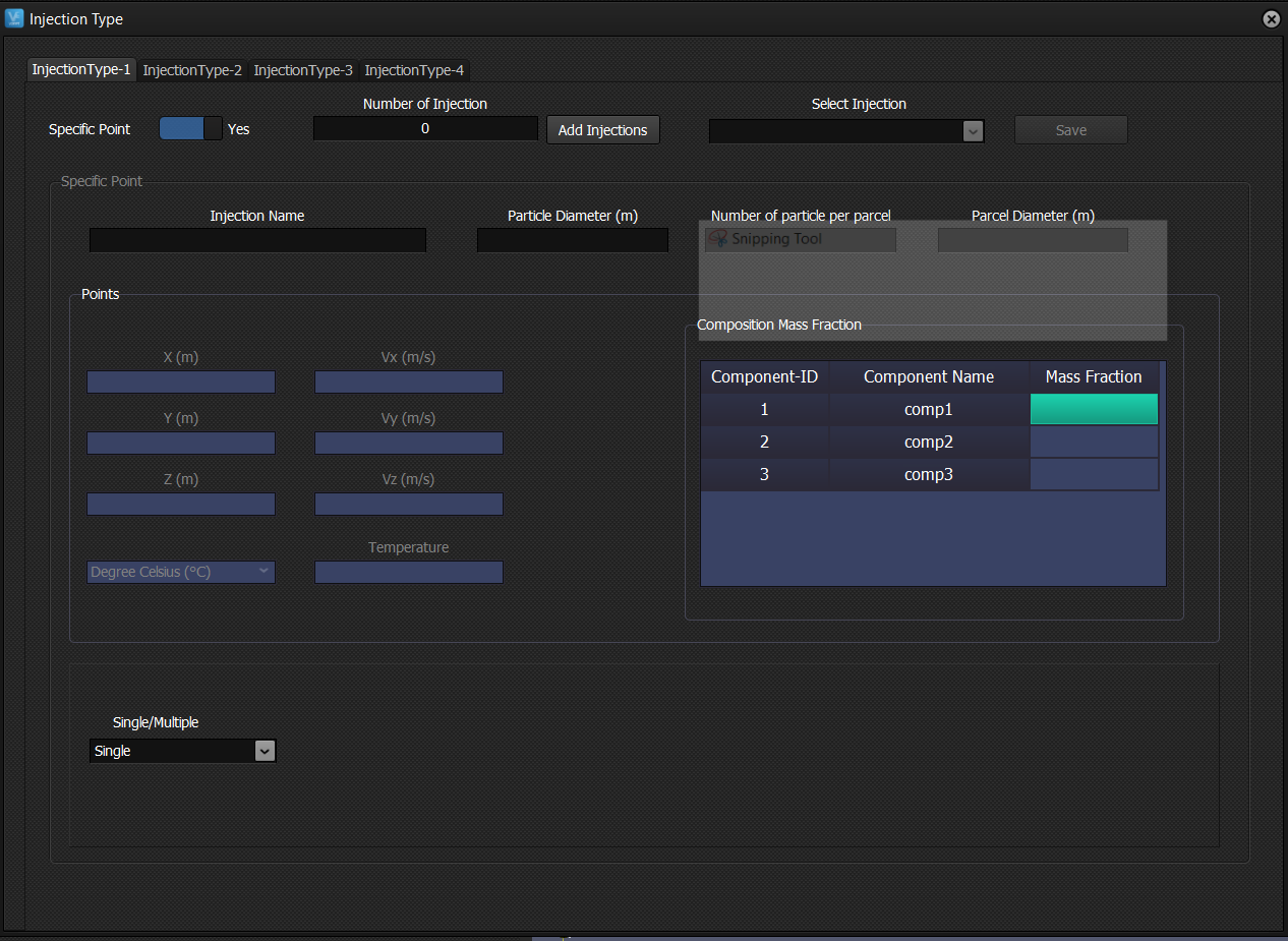
On the Main UI, select ‘Injection Initialization’ from the left pane. This causes a dialog box to open that has the 4 above mentioned injection tabs. The first tab to appear is the ‘Injection type 1’ tab as shown in Fig. 5.3.If this injection option is to be used then the provided switch needs to be turned on. When turned on many number of injection detail input check boxes appear in the dialog boxUsing the ‘Add Injection’ button new injection points can be added. ‘Number of injection’ check box shows the added injection points. Each injection needs to be added with all the remaining particle properties.First particle diameter dimensions need to filled. This activates the points data where the position, velocity and temperature properties are to be set. This further activates the the composition check box which also needs to be filled. Note that if any information is missed or not filled the setting cannot be saved.On saving individual injection setups are saved and the user can move on to create more injections in similar way.

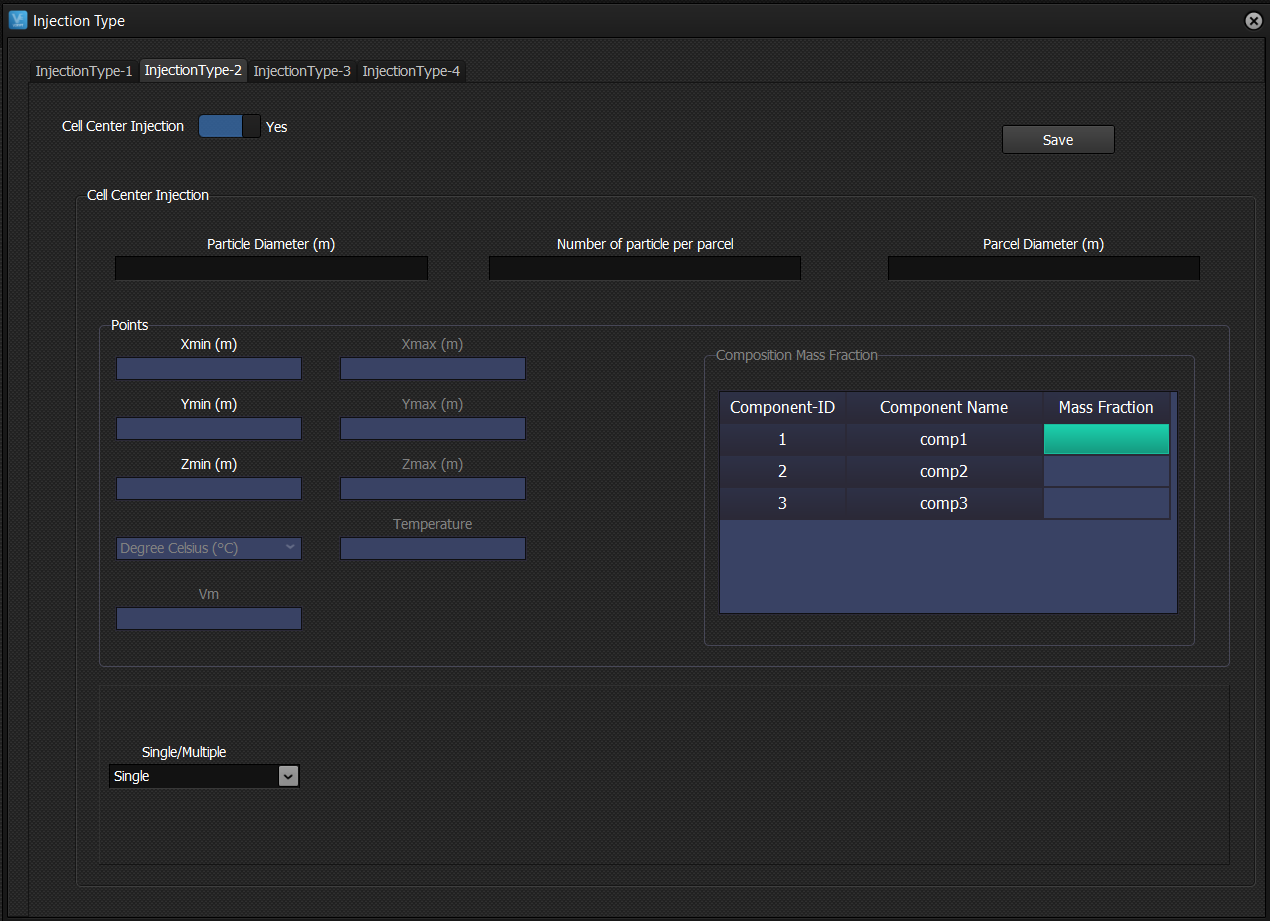
Fig. 5.3: UI design for injection type 1 and its settingIn a similar way, Injection type 2 can also be activated using the ‘Cell centre injection’ switch on the ‘Injection type-2’ tab. The input settings are similar to ‘Injection type-1’ with fundamental difference in points specification where position minimum and maximum are set. Fig. 5.4 shows the details of this setting when switched on. Similar to previous injection type single and multiple settings can also be activated for defining injection type.In case of ‘Injection type-3’ the switch besides ‘Fixed grid injection’ on the ‘Injection type-3’ tab needs to be activated to use it. Similar to previous injection the minimum and maximum position needs to be specified here also. Additionally, the distance between injection points needs to be specified here as the pitch. This variable is necessary to set in the grid density structure in the domain. Note that the maximum positions can also be switched instead to provide the directional number of particles. Thus the user is free to set precise number of injections in each direction at the provided pitch. Fig. 5.5 shows this injection type.

Fig. 5.4: UI design for injection type 2 (cell centered injection) and its setting

Fig. 5.5: UI design for injection type 3 (Fixed square grid injection) and its settingIn case of ‘Injection type-4’ the switch besides ‘Channel injection’ on the ‘Injection type-4’ tab needs to be activated to use it. Similar to ‘injection type-1’ multiple injection channels can be introduced using this. The centre position of the channel and the pitch needs to be provided here for setting the injection position. Notice that this injection type is by default a multiple or continuous injection type. So, mass flow rate needs to be set. Multiple stream injections can be set for this injection type. This injection type is also provided with standard deviation setting for particle size so that size distribution can also be set.

Fig. 5.6: UI design for injection type 4 (Feed stream channel injection) and its setting

7 . Fluid Flowsolver

7.1 Description and theory:

7.1.1 Single phase Eulerian flow model:

\frac{\partial}{\partial t} (ε_{m} ρ_{m}) + \nabla ∙ (ε_{m} ρ_{m} {\vec{u}}_{m}) = S_{m}

( 8.1)Where, the suffix m denotes the mixture of all fluid species of a single phase in the system which are modeled as Eulerian continuous phase. This fluid phase is typically a liquid or gas phase. The source term

S_{m}

represents the exchange of mass with the Lagrangian particulate or any source defined by the user. If the fluid phase exchanges mass with particle phase by water/liquid vaporization then the exchange is mapped between the Eulerian and Lagrangian grid using a grid mapping function. This relationship is given by;

S_{m} = - \sum_{p \in c e l l} S_{p} δ (\vec{r_{c}} - \vec{r_{p}})

(8.2)Where,

S_{p}

is the source term for individual particles belonging to the given cell which has been discussed in Section __. The

δ (\vec{r_{c}} - \vec{r_{p}})

is the mapping function that collects all Lagrangian particlesbelonging to the given Eulerian grid cell.The momentum equation representing for all fluid species is given by;

\frac{\partial}{\partial t} (ε_{m} ρ_{m} {\vec{u}}_{m}) + \nabla ∙ (ε_{m} ρ_{m} {\vec{u}}_{m} \vec{u}_{m}) = - ε_{m} \nabla ∙ P - \nabla ∙ \{ε_{m} μ_{m} (\nabla {\vec{u}}_{m} + \nabla {\vec{u}}_{m}^{T})\} + (ε_{m} ρ_{m} \vec{g}) + S_{m, d}

(8.3)Where;

S_{m, d}

is the source term for the drag force interaction between particle and fluid phase. The Lagrangian particle momentum are mapped onto the Eulerian grid using the 𝛿 function. The interaction force acting on the fluid grid 𝑆𝑚,𝑑 due to particles is given by;

S_{m} = - \sum_{p \in c e l l} {\vec{F}}_{p, d r a g} δ (\vec{r_{c}} - \vec{r_{p}})

(8.4)Where, the drag force on individual particles

{\vec{F}}_{p, d r a g}

are accumulated onto the discretized Eulerian grid cell points with a smoothed Diriac-delta function.

7.1.2 Single phase Eulerian energy model:

The individual fluid species modeled as scalar transport are given by;

\frac{\partial}{\partial t} (ε_{m} ρ_{m} C_{p, m} T_{m}) + \nabla ∙ (ε_{m} ρ_{m} {\vec{u}}_{m} C_{p, m} T_{m}) = \nabla ∙ (ε_{m} k_{m} \nabla T_{m}) - S_{m, E}

( 8.5)Where;

C_{p, m}

is the mean heat capacity and

k_{m}

is the mean thermal conductivity of mixture fluid belonging to the Eulerian cell.

S_{m, E}

is the energy source term for the fluid phase. This equation assumes that the heat capacity of the gas mixture is constant. The above equation can also be expressed in terms of enthalpy where;

H_{m} = ε_{m} ρ_{m} C_{p, m} T_{m}

( 8.6)

S_{m, E} = - \sum_{p \in c e l l} (h_{p} A_{p} (T_{m} - T_{p}) + S_{p, W l, v a p} λ_{W, v a p}) δ (\vec{r_{c}} - \vec{r_{p}})

(8.7)

7.1.3 Single phase Eulerian species model:

The individual fluid species modeled as scalar transport are given by;

\frac{\partial}{\partial t} (ε_{m} ρ_{m} Y_{i}) + \nabla ∙ (ε_{m} ρ_{m} {\vec{u}}_{m} Y_{i}) = S_{m}

( 8.1)The species mass fraction denoted by 𝑌𝑖 sum up to 1.0 for the fluid phase;

\sum Y_{i} = Y_{w v} + Y_{a} = 1.0

(8.4)

S_{m} = - \sum_{p \in c e l l} (K_{w, p} (Y_{W v} - Y_{W v}^{e q})) δ (\vec{r_{c}} - \vec{r_{p}})

(8.7)Where;

K_{w, p}

is the mass transfer by vaporization coefficient for water at the particle surface. Since this is also a fluid-particle transfer it has a Dirac delta mapping function.

Y_{W v}^{e q}

is the equilibrium vapor composition at the gas-particle interface.

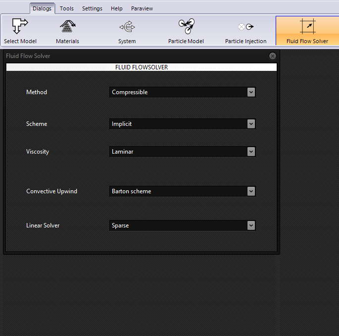
Fig. 9.1: Fluid Flowsolver selection pane for solver setting and its specific schemes.

7.2 Setting up:

On the UI upper pane, select ‘Fluid flowsolver’. This gives the selection pane on the left pane to make fluid flowsolver model choices and settings as shown in Fig. 8.1.The selections include Method (compressible or incompressible), Scheme (implicit or explicit), viscosity (Laminar or any turbulence model), convective upwind scheme and linear solver.

8 . Eulerian Boundary Condition

8.1 Description and theory:

The unstructured grid domain elements consist of cell external faces that may have been designed to have both external and internal boundaries. The boundaries are defined limits of the domain that can have or represent different conditions for the finite domain. Some of the conventional boundary types defined across CAE formats is listed in table 1. Typically in pressure-velocity based CFD solvers the boundary conditions are imposed on pressure, normal and tangential velocities. The table provides the settings for these conditions for various boundaries. The suffix ‘b’ represents the boundary cell condition and suffix ‘c1’ represents the first internal cell to boundary. In case of vector variables normal and tangential direction vector variables are represented as suffix ‘n’ and ‘t’.

Boundary Id	Boundary Name	settings
3	wall	P_b = P_c1; U_b_,n = 0; U_b_,t = -U_c1_,t;
4	pressure - inlet, inlet - vent, intake - fan	P_b = P_set; U_b,n = eval; U_b,t = U_c1,t;
5	pressure - outlet, exhaust - fan, outlet- vent	P_b = P_set; U_b,n = eval; U_b,t = U_c1,t;
7	symmetry	-
8	periodic - shadow	-
9	pressure - far - field	P_b = P_c1; U_b,n = eval; U_b,t = U_c1,t;
10	velocity - inlet	P_b = P_c1; U_b,n = U_set; U_b,t = U_c1,t;
12	periodic
14	fan, porous - jump, radiator
20	mass flow - inlet	P_b = P_c1; U_b,n = m_set/ρ_f; U_b,t = U_c1,t;
24	interface
31	parent(hanging node)
36	Outflow	P_b = P_c1; U_b,n = eval; U_b,t = U_c1,t;

8.2 Setting up:

On the UI upper pane, select ‘Boundary condition’. This gives the selection pane on the left pane to make fluid flowsolver model choices and settings as shown in Fig. 8.1.The selections include Method (compressible or incompressible), Scheme (implicit or explicit), viscosity (Laminar or any turbulence model), convective upwind scheme and linear solver..

9 . Execute

9.1 Description and theory:

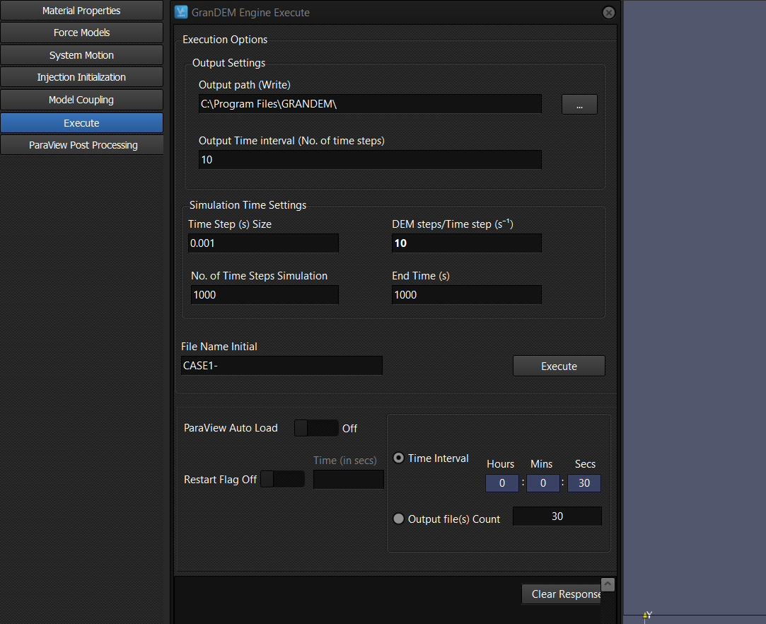
The execute is the final property to be edited before running a simulation. Fig. 7.1 shows the middle pane that is observed on clicking the Execute in the left pane. Here the output settings, time step settings, end time settings and autoload visualization settings are made. The time step size and DEM time step size are related where the DEM time step size needs to be integer greater than 1. The DEM time step here represents the individual time step over which collision particle tracking integration is performed. However, updating of all other forces is performed at the end of time step size only. This is simply because typically in DEM simulations the collision tracking needs to be refined depending on spring dashpot collision time limitations. Therefore, the time step size for other force updation is typically some factor higher than the DEM collision time step size. The other important variable setting is the number of timestep simulation and end time which are both related. Hence they autoset when the other is changed.

9.2 Setting up:

The output path and output time interval needs to be set using the check boxes at the top. The output path is the path where the output data will be written.Check boxes for time step size, DEM steps/Time step, Number of time step simulations and End time have been provided in the center of the middle pane with the heading ‘Simulation time settings’.

Fig. 7.1: The Execute selection from left tab showing the input setting details in the middle pane.Further, a setup for auto paraview visualisation loading is provided so that the user can get an auto visualization of the data while the simulation is running. This feature can be switched on by the user using the ‘Paraview Auto Load’ switch while setting the autoload timings using the check boxes besides ‘Time Interval’.In the event of a simulation crash or end of simulation, the user can also restart the simulation directly from where it stopped. This can be done by first switching on the restart switch and setting the time of restart.

10 . FILE, EDIT, SOURCE, FILTERS, AND HELP

10.1 Description and theory:

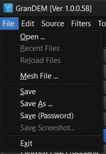
In the upper left corner of the UI interface is provided with a series of selection for miscellaneous operations and features like FILE, EDIT, SOURCE, etc. The ‘FILE’ selection has options like ‘Open’, ‘Open Mesh File’, ‘Save’, ‘Save As’ and ‘Exit’. The GRANDEM UI ‘Open’ feature can be used to import any standard Grandem case file ‘.gdm’. Similarly, it can also be used to save case ‘.gdm’ file including with password protection. The mesh file can be used to import standard fluent mesh ‘.msh’ file and replace it into the model settings.

Fig 8.1: Selection within ‘FILE’

11 Paraview Post Processing

11.1 Description and theory:

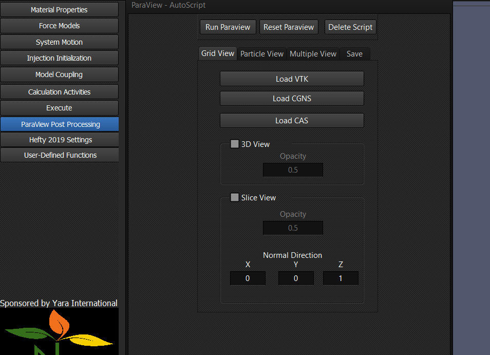
This selection on the left pane is used after a simulation run has completed and output result data is available for paraview post-processing and visualization study. On selecting this the middle pane appears as shown in Fig. 9.1. Here in this feature various data type files can be loaded into and viewed in paraview. This includes .cgns, .vtk and .cas fluent files for the grid and fluid data while .vtu files for the particle data.In the middle pane 3 main buttons have been provided to start paraview, reset paraview and delete script. Below this are 4 tabs each having their individual post processing functionalities. The first tab is ‘Grid view’ tab for loading grid and fluid data. The second tab is ‘Particle view’ tab for loading particle data files. The third tab is ‘Multiple View’ tab used for expanding to multiple views of the prevailing view to show velocity field, thermal field and species field.

Fig 9.1: The ParaView Post Processing selection from left tab showing the input setting details in the middle pane.

11.2 Setting up:

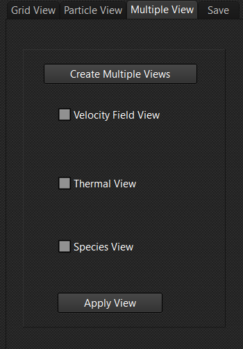
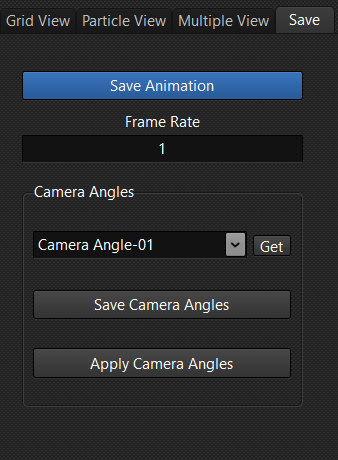
Check if paraview has been started. If not start paraview by clicking the button ‘Run Paraview’.The first tab ‘Grid view’ can be seen in Fig. 9.1 where 3 buttons have been provided to load either vtk, cgns or cas files. By selecting the check box ‘3D view’ and/or ‘Slice view’ Opacity and slice plane direction can be set before loading.When any of the ‘load’ button is clicked a selection dialog box opens to browse to the folder that contains the data files. Browse to the location folder and select the folder to press ok. This loads the data files into paraview.Move to the ‘Particle View’ tab where on clicking Load VTU button a dialog box opens to browse the data folder location. Browse to the data file location where .pvd file can be located. Select the .pvd file and click ‘open’. This loads particle data files.The next tab is ‘Multiple view’ tab that is utilized when multiple view are to be created simultaneously. This tab has the button ‘Create Multiple views’ (Fig. 9.2) that on clicking creates 4 render views.This tab further has check boxes for ‘velocity field view’, ‘thermal view’ and ‘species view’ all of which can be selected based on user requirement. The ‘Apply view’ button sets up the parallel views of the selected views in the check boxes.The ‘Save’ tab has the functionality to save animations after setting frame rate for the video as show in Fig. 9.3. Besides, this tab also has camera angles saving functionality that sets and saves camera view angles with specific names by clicking the ‘Save Camera Angles’ button.The saved camera angles can be used to select from the drop down menu. When the ‘Apply Camera Angles’ button is used the selected camera angle view is shown or presented. This button can be used for resetting back to a specific angle that the user wants to set.

Fig. 9.2: Multiple view tab and settings. Fig. 9.3: Save tab and settings.

📘 Contents